– Introduction to Graphs 2
![]() WARNING: Caliach standard support is limited to the operation of the Graphs 2 framework within Caliach Vision. The contents of Graphs 2 and their design is specifically excluded from normal subscription support. Similarly, Caliach can give help with design of Graphs but only as a chargeable service.
WARNING: Caliach standard support is limited to the operation of the Graphs 2 framework within Caliach Vision. The contents of Graphs 2 and their design is specifically excluded from normal subscription support. Similarly, Caliach can give help with design of Graphs but only as a chargeable service.
Graphs 2 is a second generation Graphing tool embedded in Caliach Vision. With this you can generate X-Y charts, Pie charts, Polar charts and Meter charts and embed these in windows and/or reports.
Designs of graphs are self-contained and stored in the datafile (XMLFILE) and their use may be restricted to specific users or groups. Data collection is typically carried out by one or more Data Views. Because they are complex and can be onerous to design, Caliach has provided a Web Server Collection on the Support area of www.caliach.com. Graph designs can be downloaded and modified for your use from within Caliach Vision. Your designs can be uploaded to this collection to provide a pool of designs that all can use painlessly.
![]() NOTE: This system exploits the Omnis Studio Graph2 component which in turn is based on a graphing engine (called ChartDirector from Advanced Software Engineering Ltd) and was introduced in order to simplify graphing functionality in Omnis. The Graph2 component can produce many more types of chart and is easier to use than the old Graph component, which for backwards compatibility is still available in Omnis and Caliach Vision, but is no longer maintained or supported.
NOTE: This system exploits the Omnis Studio Graph2 component which in turn is based on a graphing engine (called ChartDirector from Advanced Software Engineering Ltd) and was introduced in order to simplify graphing functionality in Omnis. The Graph2 component can produce many more types of chart and is easier to use than the old Graph component, which for backwards compatibility is still available in Omnis and Caliach Vision, but is no longer maintained or supported.
Graph designs are saved, uploaded and downloaded as XML data or files containing all the structures needed but with no collected data. Data Views can, however, store the data they collect.
Types of Graphs
There are 4 major types of graphs: X-Y Charts, Pie Charts, Polar Charts and Meters and Gauges. and other than Pie Charts each major type has several minor types of chart.
The Sample data shows the form in which the data can be applied in comma-delimited lines of data points. This will then be converted into a list and passed to the graph. More typically you would design a Data View that would return a list in the appropriate form for your graph.
X-Y Charts
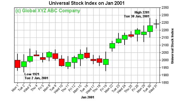
X-Y Charts have the following minor types:
|
Minor Type |
Simple Example |
|---|---|
|
Bar Chart |
|
|
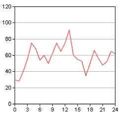
Line Chart |
|
|
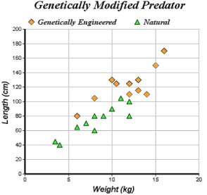
Scatter Charts |
|
|
Area Charts |
|
|
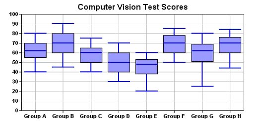
Box Whisker Charts |
|
|
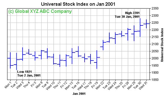
High/Low/Open/Close Charts |
|
|
Candlestick Charts |
|
Pie Charts
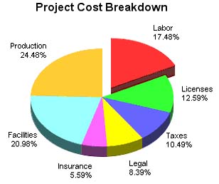
Pie Charts do not have minor types. The data in a pie chart is represented as sections, or slices of a pie. Pie charts may not have minor types but have numerous visual effects.
|
Pie Chart |
|
Polar Charts
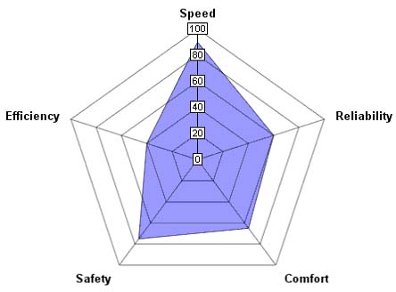
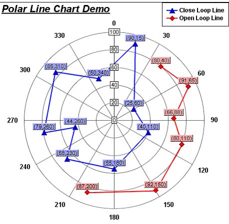
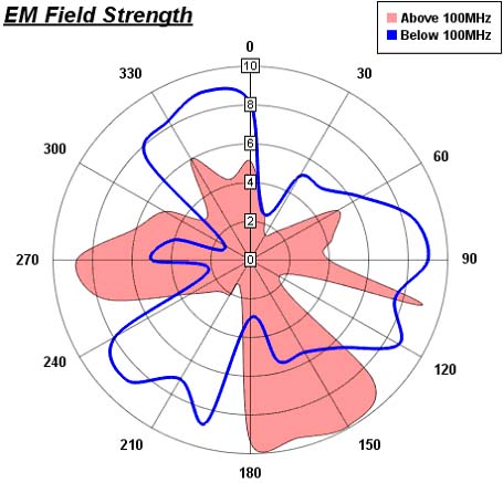
Polar charts represent data points on a radial axis with the values represented as the distance from the centre. Four minor types are available.
|
Minor Type |
Simple Example |
|---|---|
|
Polar Area |
|
|
Polar Line |
|
|
Polar Spline Line and Area |
|
Meters and Gauges
Meter charts represent numeric measurements. Two minor types are available.
|
Minor Type |
Simple Example |
|---|---|
|
Linear – vertical or horizontal |
|
|
Radial |
|
Where Graphs are Used
The most obvious place graphs can be used is in Key Performance Indicators to provide graphical performance and warning data on a regular and timely manner.
In addition, they can be included on custom windows and reports.
Data Sources
Data can be supplied in a number of forms to a graph as follows:
1. Data View Name
If you enter a Data View name, then the Data View will be run and it’s data will populate the graph. In Data Layers you can have more than one Data View, separating them with a carriage-return.
2. Comma-delimited Data or Actual Numeric Values
It there is a comma in the text entered the graph will assume that this is data to be applied. So for fixed data, perhaps copied from a spreadsheet, comma-delimited values can be used to populate data. For single value data elements, such as Pointer values or Zone ranges, single simple numbers can be used.
3. Square-bracket Notation
An Omnis Studio expression enclosed in square-brackets can be used as data. This is useful for single-value items, or multiples only by separate square-bracket expressions, and can contain any calculation or function that can be interpreted within the scope of the Data View object.
For example, [#D] will be replaced by the current data, [#T] the current time and [Data.L1.2.3] is dot-notation for the value of the third cell in the second row of the by the data list generated by the main layer zero data source. For Extra fields the syntax would be [Extra.L1.2.3]. You can use any resolvable function, for example:
[$ctask.tLangSwap.$lookupIDX(con('1',Data.L1.2.3),'fr')]
would return the French language swap translation of the part index code 1 description for the data in L1.2.3.
Square-bracket notation can also be used in titles and other textual elements of the graph, as well as Extra Fields described in the section below. And the full list of available data element are as follows:
|
Full Syntax |
Description |
Examples |
|---|---|---|
|
Data.L1.row.column |
The main graph data in sequence of source and layer. So layer 0’s first data set or Data View data will be Data.L1.., the next will be Data.L2.. progressing up the layers. So if you have 4 layers and a total of 6 Data Views you will have Data.L1 through Data.L6. The structure of the data is a list of lists of varying arrays. |
[Data.L1.1.1] is the data in the 1st column on the 1st row of the 1st Data source. |
|
Extra.L1.row.column |
Similar to the Data list in order if Data Views in Extra Fields of layers. The structure of the data is a list of lists of varying arrays, as in Data. |
[Extra.L4.3.2] is the data in the 2nd column on the 3rd row of the 4th Data Extra Fields source. |
|
Mark.row.1 |
This is the data from Marks derived from Data Views. This is a simple list with one column so the only values from multiple Marks are Mark.1.1, Mark.2.1, Mark.3.1, etc. For the final column entry you can either use the 1 or the name of the column which value in lower case. |
[Mark.1.1] is the data value from the 1st Mark. |
|
Zone.row.column |
This is the data from extra Zones derived from Data Views. This is a simple list with two columns, one for the lower value and one for the upper, so the values from multiple Zones are Zone.1.1 and Zone.1.2, then the next Zone is Zone.2.1 and Zone.2.2, etc. For the final column entry you can either use the number or name of the column, lower or upper. |
[Zone.1.1] or [Zone.1.lower] is the lower data value from the 1st Zone. |
|
Pointer.row.1 |
This is the data from extra Pointers derived from Data Views. This is a simple list with one column so the only values from multiple Pointers are Pointer.1.1, Pointer.2.1, Pointer.3.1, etc. For the final column entry you can either use 1 or the name of the column which is value. |
[Pointer.1.1] is the data value from the 1st extra Pointer. |
4. Nothing
This applies only to the Data of a Data Layer. When this is left blank demonstration data is used appropriate for the Major and Minor graph types. This is useful when you are designing the layout of a graph, before you have sorted out the data to be used.
5. % Syntax
This applies to single value items, for instance, zones that normally accept a single numeric value. If you append a %, the graph will calculate the absolute value based on the percent of the full amount.
Extra Fields
While the Data Layer is drawn from the Data source defined above, you can also add a list of extra data that can be referenced in the labels or custom data labels using the syntax described below in the Parameter Substitution and Formatting section below.
Extra fields are only useful for labels of one form or another and using the correct syntax.
Square-bracket notation can be used and is interpreted in two ways:
Each Extra Field can be a different expression or a mix of text, values and square bracket expressions, for example, [#D],Tomorrow,Next Day,Whenever.
A series line that consists of a single square-bracket expression will lead the program to replicate the expression for each data element of the series. And this in turn has a super-syntax of {value} (note the curly-brackets) to reference the underlying data of the data-point the extra field is referring to. So:
[pick(mod({value},12)=0,'','*')]
would make every 12th data point extra field equal to *, to indicate a new year, perhaps. Or even more picturesquely the following would place the symbols ◔ ◑ ◕ ● represent quarters using Unicode characters:
[pick(mod({value},4),unichr('U+25D4'),unichr('U+25D1'),unichr('U+25D5'),unichr('U+25CF'))]
Assuming, of course, that the font can handle such characters!
Parameter Substitution and Formatting
Charts often contain a lot of text strings, such as sector labels in pie charts, axis labels for XY charts, data labels for the data points, graph titles, and so on. You can substitute many of these parameters to allow you to configure precisely the information contained in the text and their format. For example, when drawing a pie chart with side label layout, the default sector label format is:
{label} ({percent}%)
In drawing the sector labels, the graph will replace {label} with the sector name, and {percent} with the sector percentage. So the label will be something like:
ABC (34.56%)
You can change the sector label format by changing the format string. For example, you can change it to:
{label}: US${value}K ({percent}%)
The sector value will then be something like:
ABC: US$123K (34.56%)
For fields that are numbers, dates, or times, the Graph feature supports a special syntax in parameter substitution to allow formatting of these values. Please refer to the Number Formatting and Date/Time Formatting sections below for details.
The following tables describe the fields available for various chart objects.
Parameters for Pie Charts
|
Parameter |
Description |
|---|---|
|
sector |
The sector number. The first sector is 1, the second is 2, and so on. |
|
label |
The text label of the sector. |
|
value |
The data value of the sector. |
|
percent |
The percentage value of the sector. |
Parameters for all XY Charts
The following are parameters that apply to all XY Chart layers in general. Some layer types may have additional parameters (see below).
Note that some parameters do not apply in certain cases. For example, when specifying the aggregate label of a stacked bar chart, the {dataSetName} parameter does not apply, because a stacked bar is composed of multiple data sets. It does not belong to any particular data set and hence does not have a data set name.
|
Parameter |
Description |
|---|---|
|
x |
The x value of the data point. |
|
xLabel |
The bottom x-axis label of the data point. |
|
x2Label |
The top x-axis label of the data point. |
|
value |
The value of the data point. |
|
accValue |
The accumulative value of the data point. This is useful for stacked charts, such as stacked bar chart and stacked area chart. |
|
totalValue |
The total value of all data points. This is useful for stacked charts, such as stacked bar chart and stacked area chart. |
|
percent |
The percentage of the data point based on the total value of all data points that are in the same x position and same data group as the current data point. This is useful for stacked charts, such as stacked bar chart and stacked area chart. |
|
accPercent |
The accumulated percentage of the data point based on the total value of all data points. This is useful for stacked charts, such as stacked bar chart and stacked area chart. |
|
gpercent |
The percentage of the data point based on the total value of all data points. |
|
dataSet |
The data set number to which the data point belongs. The first data set is 1, the second is 2, and so on. |
|
dataSetName |
The name of the data set to which the data point belongs. |
|
dataItem |
The data point number within the data set. The first data point is 1, the second is 2, and so on. |
|
dataGroup |
The data group number to which the data point belongs. The first data group is 1, the second is 2, and so on. |
|
dataGroupName |
The name of the data group to which the data point belongs. |
|
layerId |
The layer number to which the data point belongs. The first layer is 1, the second is 2, and so on. |
|
fieldN |
The (N + 1)th extra field. For example, {field0} means the first extra field, and {field1} means the second extra field. {fieldN} means the extra field is indexed by the data point number. The Pth data point corresponds to the Pth element of the extra field. |
Additional Parameters for HLOC and CandleStick Layers
|
Parameter |
Description |
|---|---|
|
high |
The high value of the data representation. |
|
low |
The low value of the data representation. |
|
open |
The open value of the data representation. |
|
close |
The close value of the data representation. |
Additional Parameters for Box Whisker Layers
|
Parameter |
Description |
|---|---|
|
top |
The value of the top edge of the box-whisker symbol. |
|
bottom |
The value of the bottom edge of the box-whisker symbol. |
|
max |
The value of the maximum mark of the box-whisker symbol. |
|
min |
The value of the minimum mark of the box-whisker symbol. |
|
med |
The value of the median mark of the box-whisker symbol. |
Additional Parameters for Trend Layers
|
Parameter |
Description |
|---|---|
|
slope |
The slope of the trend line. |
|
intercept |
The y-intercept of the trend line. |
|
corr |
The correlation coefficient in linear regression analysis. |
|
stderr |
The standard error in linear regression analysis. |
Parameters for Polar Charts
|
Parameter |
Description |
|---|---|
|
radius |
The radial value of the data point. |
|
value |
Same as {radius}. See above. |
|
angle |
The angular value of the data point. |
|
label |
The angular label of the data point. |
|
name |
The name of the layer to which the data point belongs. |
|
i |
The data point number. The first data point is 1, the second is 2,and so on. |
Parameters for an Axis
|
Parameter |
Description |
|---|---|
|
value |
The axis value at the tick position. |
|
label |
The axis label at the tick position. |
Number Formatting
For parameters that are numbers, the Graph function supports a number of formatting options in parameter substitution.
You follow the name of the parameter with a vertical bar character and then the format codes. For example, if you want a numeric field {value} to have a precision of two digits to the right of the decimal point, use , (comma) as the thousand separator, and use . (dot) as the decimal point, then you should use {value|2,.}. The number 123456.789 will therefore be displayed as 123,456.79.
For numbers, the formatting options are specified using the following syntax:
{[param]|[a][b][c][d]}
where:
|
Parameter |
Description |
|---|---|
|
[param] |
The name of the parameter. |
|
[a] |
An integer specifying the number of digits to the right of the decimal point. The default is automatic. To use the default, simply skip this parameter. |
|
[b] |
The thousand separator. Should be a non-alphanumeric character (not 0-9, A-Z, a-z). Use ~ for no thousand separator. |
|
[c] |
The decimal point character. |
|
[d] |
The negative sign character. Use ~ for no negative sign character. |
You may skip the trailing formatting options if they are not needed. For example, {value|2} means formatting the value with two digits to the right, where the thousand separator, decimal point character, and negative sign character are all using the default settings of the chart.
Date/Time Formatting
For parameters that are dates and or times, the formatting options can be specified using the following syntax (note the parameter name is followed by a vertical bar character):
{[param]|[datetime_format_string]}
where [datetime_format_string] must start with an alphabetic character (A-Z or a-z), and may contain any characters except ). Certain characters are substituted according to the following table:
|
Characters |
Description |
|---|---|
|
yyyy |
Year in 4 digits (e.g. 2005) |
|
yyy |
Year showing only the least significant 3 digits (e.g. 007 for the year 2007) |
|
yy |
Year showing only the least significant 2 digits (e.g. 07 for the year 2007) |
|
y |
Year showing only the least significant 1 digit (e.g. 7 for the year 2007) |
|
mmm |
Month formatted as its name. The default is to use the first 3 characters of the English month name (Jan, Feb, Mar, etc.). |
|
mm |
Month formatted as 2 digits from 01 – 12, with leading zero if necessary. |
|
m |
Month formatted using the minimum number of digits from 1 – 12. |
|
dd |
Day of month formatted as 2 digits from 01 – 31, with leading zero if necessary. |
|
d |
Day of month formatted using the minimum number of digits from 1 – 31. |
|
w |
The name of the day of week. The default is to use the first 3 characters of the English day of week name (Sun, Mon, Tue, etc.). |
|
hh |
The hour of day formatted as 2 digits, adding leading zero if necessary. The 2 digits will be 00 – 23 if the a option (see below) is not specified, otherwise it will be 00 – 12. |
|
h |
The hour of day formatted using the minimum number of digits. The digits will be 0 – 23 if the a option (see below) is not specified, otherwise it will be 0 – 12. |
|
nn |
The minute formatted as 2 digits from 00 – 59, adding leading zero if necessary. |
|
n |
The minute formatted using the minimum number of digits from 00 – 59. |
|
ss |
The second formatted as 2 digits from 00 – 59, adding leading zero if necessary. |
|
s |
The second formatted using the minimum number of digits from 00 – 59. |
|
a |
Display either am or pm, depending on whether the time is in the morning or afternoon. |
For example, a parameter substitution format of {value|mm-dd-yyyy} will display a date as something similar to 09-15-2002. A format of {value|dd/mm/yy hh:nn:ss a} will display a date as something similar to 15/09/02 03:04:05 pm.
External Files (Images and Fonts)
Images
Graphs can use externally stored image files: png, jpg, jpeg, gif, wbmp or wmp (case insensitive) and should have these file suffixes. They must be located in the GraphsImages folder in the same directory as the Vision.lbs Caliach Vision library. If this folder does not exist Caliach Vision will create it.
Besides the graph wallpaper, images can be used in text using CDML; so the following will insert the snowy.png image:
This is snowy <*img=snowy.png*>

Note that in the example above the Wallpaper file has also been set to a small identity graphic with Caliach in 15% grey. Using a graphic form that supports transparency permits this effect, for example .png.
Fonts
Because Graphs is an an external component it does not use normal fonts used in Caliach Vision’s reports and windows.
Graphs can use any true type (.ttf) or true type collection fonts (.ttc) and they must be located in the Fonts folder in the same directory as the executing Omnis Studio. If that Font folder does not exist you can create it.
If you want to use a font that is not currently in the Fonts folder, you must add it. After you add it when you next open the Graph will be listed in the font list.
In the design Graphs 2 Properties window there is a final Files tab pane in which you can list the extra files needed by the graph. This includes Fonts and Images. This list enables the system to subsequently manage these files around the network for other users. After you have finished the design, you can use the Synchronise Files List to Design to create or update the list of external files the design uses. When you save the graph design, these files will be copies from the extra files cache on the server or to it so that these files are available to all potential users. See below for how the file cache works.
Any text elements and labels can use a type of Mark Up Language (supported in the underlying graph engine and called ChartDirector Mark Up Language (or CDML) to include formatting information in text strings by marking up the text with tags. This Mark Up Language allows a single text string to be rendered using multiple fonts, with different colours, and even embed images in the text. CDML is supported in all text objects including chart titles, legend keys, axis labels, data labels, and so on. For example:
<*font=timesi.ttf,size=18,color=FF0000*>Italic red text<*font=arial.ttf,size=10,color=8000*> and normal text
![]()
Note the American spelling of colour is used.
Extra Files Server Cache
To reduce network traffic extra fonts and images are stored locally to the executing Omnis Studio and Caliach Vision respectively. However, as many users may want to use the graph designs these files are copied to a GraphCache folder alongside your datafile (or in the case of ODB, the Direct Path folder). Within GraphCache there are the _fonts and _images folders that contain copies of extra files on all graphs designed on the site. If you download graphs from www.caliach.com web server and new files will be added.
![]() WARNING: Uploading Fonts and Images can be an infringement of copyright. Caliach can not be responsible for your breaching copyright.
WARNING: Uploading Fonts and Images can be an infringement of copyright. Caliach can not be responsible for your breaching copyright.
When a user uses a graph for the first time the program automatically copies files from the server cache to the users local folders, if they are not already there.
![]() TIP: This system does not refresh changed image files, so if you want to change an image file, change it manually in the server cache folder, and delete the local copies so that they are renewed when the graph is next run.
TIP: This system does not refresh changed image files, so if you want to change an image file, change it manually in the server cache folder, and delete the local copies so that they are renewed when the graph is next run.
| See also: – |
Compiled in Program Version 5.10. Help data last modified 6 Jun 2012 03:50:00.00. No class.


